Calculation Methodology
A multiyear projection is a mathematical model that takes an assumed status quo, the base year, and projects future years by making modifications for locally known assumptions.
Each year is calculated based on the result of the prior year:
- Determine the starting value for the projected year. In 'Year 2,' the prior year is the 'Base Year' plus 'Adjustment.' For other projected years, it is the prior year value.
- Apply the assumptions in the order listed. Note: The processing order will impact the final estimate when the assumptions applied include both dollar-based and percentage-based values.
- Determine the ending value for the projected year.
- Repeat steps 1-3 to project subsequent years.
Assumptions displayed in the Base Year column are for informational purposes only.
Example 1 - Status Quo
The base year budget for an object is $100. There is a manual adjustment to the base year budget of $10, for a total adjusted base year budget of $110.
No assumptions are applied to the object, so the projected years are at status quo, or $110 for Year 2 and Year 3.
| Description | Year 2 | Year 3 |
|---|---|---|
| 1. Starting Value | $110.00 | $110.00 |
| 2. Apply the first assumption | none | none |
| 3. Determine the ending value | $110.00 | $110.00 |
| 4. Repeat Steps 1 - 3 | (see Year 3 column) | end |

Example 2 - Apply Two Assumptions
Example 2 builds on example 1 by adding two assumptions to the object. The first assumption is a reduction of $25 for a one-time purchase that occurred in the base year and won't be repeated in Year 2 or Year 3. The second assumption is for the California consumer price index (CPI). The CPI adjustment is 4.0000% in year 2 and 3.5000% in year 3. The ending values for the object in Year 2 and Year 3, respectively, are $88.40 and $91.49.
Note: To apply a percentage assumption, first calculate then apply the equivalent dollar value based on the provided percentage.
| Description | Year 2 | Year 3 |
|---|---|---|
| 1. Starting Value | $110.00 | $88.40 |
| 2a. Apply the first assumption | - $25.00 = $85.00 | + 0.00 = $88.40 |
| 2b. Apply the second assumption | x 4.000% (or $3.40) = $88.40 | x 3.500% (or $3.09) = $91.49 |
| 3. Determine the ending value | $88.40 | $91.49 |
| 4. Repeat Steps 1 - 3 | (see Year 3 column) | end |

Example 3 - Apply Two Assumptions in Reverse
Example 3 reverses the order of the two assumptions from example 2. The ending values for the object in Year 2 and Year 3, respectively, are $89.40 and $92.53. The increased difference is that the CPI percentage is applied to a balance that includes the one-time purchase of $25.
| Description | Year 2 | Year 3 |
|---|---|---|
| 1. Starting Value | $110.00 | $89.40 |
| 2a. Apply the first assumption | x 4.000% (or $4.40) = $114.40 | x 3.500% (or $3.13) = $92.53 |
| 2b. Apply the second assumption | - $25.00 = $89.40 | + 0.00 = $92.53 |
| 3. Determine the ending value | $89.40 | $92.53 |
| 4. Repeat Steps 1 - 3 | (see Year 3 column) | end |

Example 4 - One-time in a Projected Year
In Year 2, an LEA plans to purchase three classroom sets, 90 devices, at $1,000/ea. These are the last sets to be purchased per the Technology Plan.
- To project Year 2, what adjustment is made to the base year?
Increase expenditures by $90,000.00. - To project Year 3, what adjustment is made to Year 2?
Decrease expenditures by $90,000.00. - Is it applied as a one-time or ongoing adjustmnet?
One time. The adjustment is applied and then reversed in the projection.
| Description | Year 2 | Year 3 |
|---|---|---|
| 1. Starting Value | $110,000.00 | $110,000.00 |
| 2. Apply the one-time assumption | + 90,000.00 | + 0.00 |
| 3. Determine the ending value | $200,000.00 | $110,000.00 |
| * Reverse the one-time assumptions | - 90,000.00 | -0.00 |
| Determine the starting value for subsequent year | $110,000.00 | $110,000.00 |
| 4. Repeat steps 1-3 | (see Year 3 column) | end |

Example 5 - One-time Activity in the Base Year
What if the LEA in example 4 advanced their plans and made the purchase in the base year? Assume the base year Budget has been updated for the $90,000.00 purchase.
- To project Year 2, what adjustment is made tto the base year?
Decrease expenditures by $90,000.00. - To project Year 3, what adjustment is made to Year 2?
No additional adjustment. - Is it applied as a one-time or ongoing adjustment?
Ongoing. The purchase activity is one-time in nature, but the adjustment to the projection is ongoing because the activity occurred in the base year.
| Description | Year 2 | Year 3 |
|---|---|---|
| 1. Starting Value | $200,000.00 | $110,000.00 |
| 2. Apply the one-time assumption | - 90,000.00 | + 0.00 |
| 3. Determine the ending value | $110,000.00 | $110,000.00 |
| * Reverse the one-time assumptions | Not applicable | Not applicable |
| Determine the starting value for subsequent year | $110,000.00 | $110,000.00 |
| 4. Repeat steps 1-3 | (see Year 3 column) | end |

The ongoing adjustment assumption becomes part of status quo. It is not reversed after step 3.
Example 6 - Proportional Relationship
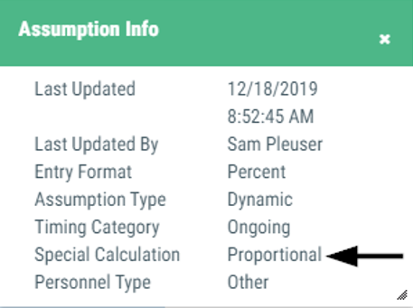
An assumption with the 'Proportional' setting first calculates the change within the resource between two fiscal years for the object range specified in the assumption, and then applies the result to project a related budget value.

Sample assumption:
- Proportional Relationship
Scenario:
The base year budget for other classified salaries is $10,000.00. Two assumptions are applied. The first is to project the salary cost of classified steps as an annual increase of 1.5% (or $150.00 in year two). The second is to project an ongoing staffing change of $1,000.00 (or 10.0000%) in year two.

The base year budget for PERS is $1,972.10. The proportional assumption increases the Year 2 budget for PERS by 11.5000% ($226.79), in proportion to the increase in classified salaries.
To project the related increased cost for PERS retirement, the Proportional Relationship assumption is applied to the PERS retirement object based on the rate of change calculated from the classified salaries object range, objects 2000-2999.
Step I - Determine the rate of change for the identified object range.
| Description | Year 2 | Year 3 |
|---|---|---|
| 1. Projected year's value for objects 2000-2000 | $11,150.00 | $11,317.25 |
| 2. Subtract the prior year's value | - $10,000.00 = $1,150.00 | - $11,150.00 = $167.25 |
| 3. Divide by the prior year's value to calculate the rate of change to be applied | ÷ $10,000.00 = 11.5000% | ÷ $11,150.00 = 1.5000% |
Step II - Apply the rate of change to the object being projected.
| Description | Year 2 | Year 3 |
|---|---|---|
| 4. Starting value of PERS | $1,972.10 | $2,198.89 |
| * Apply the rate calculated in step 3 | x 11.5000% (or $226.79) | x 1.5000% (or $32.98) |
| 5. Determine the ending value | = $2,198.89 | = $2,231.87 |
| 6. Repeat steps 1-5 | (see Year 3 column) | end |

Example 7 - Rate Change
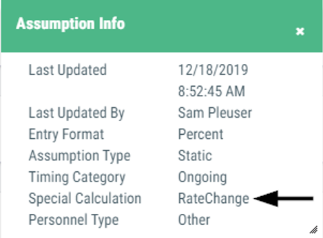
An assumption with the 'RateChange' setting first calculates the change between two percentage or dollar values entered within the assumption, and then applies the result.

Sample assumptions:
- STRS or PERS Rate Change and most other benefit related assumptions
- California Lottery - Base or Instructional Materials
- Students - TK12 and all other student assumptions
Scenario:
Continuing with the PERS benefit projection scenario in example 6, the PERS rate is projected to increase per the following schedule:
- 19.7210% Base Year
- 22.8000% Year 2
- 24.9000% Year 3
Rate change assumptions apply the calculated percent change between two dollar or percentage rates to create the projected budget.
Note that the following two calculations yield the same results. Applying the rate change assumption like the second calculation allows us more flexibility to adjust our projection with proportional or students assumptions when appropriate.
- Salaries (less excluded salaries) x new rate
$11,150.00 x 22.8000% = $2,542.20 - Prior year budget (plus assumptions) x percent change in rate
$2,198.89 x (1+[(22.8000% - 19.7210%) / 19.7210%]) = $2,542.20
Step I - Determine the rate of change between the rates specified in the assumption.
| Description | Year 2 | Year 3 |
|---|---|---|
| 1. Current year's value | 22.8000% | 24.9000% |
| 2. Subtract the prior year's value | - 19.7210% | - 22.8000% |
| 3. Divide by the prior year's value to calculate the rate of change to be applied. | ÷ 19.7210% = 15.6128% | ÷ 22.8000% = 9.2105% |
Step II - Apply the rate of change to the object being projected.
| Description | Year 2 | Year 3 |
|---|---|---|
| 4. Starting value of PERS | $1,972.10 | $2,542.20 |
| 5. Apply proportional assumption | x 11.5000% = $2,198.89 | x 1.5000% (or $38.13) = $2,580.33 |
| * Apply the rate change assumption value calculated in step 3 | x 15.6128% (or $343.31) | x 9.2105% (or $237.67) |
| 6. Determine the ending value | $2,542.20 | $2,818.00 |
| 7. Repeat steps 1-6 | (see Year 3 column) | end |

Example 8 - Manual
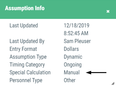
An assumption with the 'Manual' setting applies the value entered in to the assumption as the final projected result without any calculation.

Sample assumptions:
- Manual Entry
- Most special screen assumptions
- Expiring Activity
Scenario:
The LEA has an approved equipment replacement plan, including the budgeted costs allocated for a replacement schedule.
| Description | Year 2 | Year 3 |
|---|---|---|
| 1. Starting value | $25,000.00 | $30,000.00 |
| 2. Apply the manual assumption | $30,000.00 | $35,000.00 |
| 3. Determine the ending value | $30,000.00 | $35,000.00 |
| 4. Repeat steps 1-3 | (see Year 3 column) | end |

Example 9 - Zero
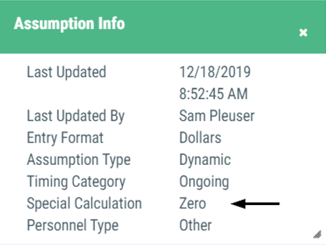
As assumption with the 'Zero' setting applies the projected value of $0 to all future years.

Sample assumption:
- Zero Out Activity
Scenario:
Altering the scenario in example 8, the LEA is discontinuing its equipment replacement plan after the current year.
| Description | Year 2 | Year 3 |
|---|---|---|
| 1. Starting value | $25,000.00 | $0.00 |
| 2. Apply the zero out activity assumption | $0.00 | $0.00 |
| 3. Determine the ending value | $0.00 | $0.00 |
| 4. Repeat steps 1-3 | (see Year 3 column) | end |
